Statistical analysis

Phonometrica provides a dedicated environment for fitting and comparing statistical models. To open an analysis, create one from a concordance or dataset using the Analyze command, or open an existing .phon-analysis file. The analysis view is divided into three areas: a top bar for entering formulas, a left panel with column and model lists, and a right panel with tabs for results, post-hoc tests, diagnostics, and exploratory plots.

Support for statistical modeling was introduced in version 0.9 and is currently classified as a preview/beta feature. The core estimation engines (covering fixed-effects Linear, Binomial, and Poisson regressions) were implemented by the lead author within the Phonometrica codebase. More specialized modules, including Negative Binomial regression, Mixed-Effects models, and Bayesian inference, along with post-hoc tests and residual diagnostics, were developed with the assistance of Claude Opus 4.6 (as of April 2026) using algorithmic guidance from established literature and reference implementations in R.

While our internal benchmarking shows an excellent match across a diverse suite of datasets when compared to reference R packages (such as lme4 or glmmTMB), these features are provided without a guarantee of absolute numerical parity, and the Bayesian engine is still considered experimental at this stage. Users may encounter minor discrepancies due to differences in optimization algorithms, convergence criteria, or numerical stability in edge cases. We strongly recommend cross-validating critical results in a secondary statistical environment for the time being. We welcome community feedback and detailed bug reports.

Top bar

The top bar contains the following elements:

• Formula: an editable text field where you enter your model formula using R-style syntax (e.g. F1 ~ vowel + context). Press Enter or click Fit to fit the model.

• Outcome: a drop-down menu to select the type of response variable: Continuous (for measurements such as formant frequencies or durations), Continuous (robust) (for continuous measurements that may contain outliers, such as formant values with tracking errors), Binary (for binary outcomes such as present/absent), Count (for count data), Overdispersed count (for count data with extra variability), or Proportion (for values strictly between 0 and 1). Hover over each option to see the corresponding statistical family and link function.

• Fit: fits the model described by the current formula and outcome type. The fitted model is added to the model list.

• Estimation: choose between Frequentist (maximum likelihood with Wald-based p-values, the default) and Bayesian (approximate Bayesian inference with weakly informative priors, reporting posterior means, credible intervals, and probability of direction). See Bayesian estimation below.

• Help (): opens this documentation page.

Formula syntax

Phonometrica uses R-style formula syntax. The left-hand side is the response variable, and the right-hand side lists the predictors separated by +.

Fixed effects

• y ~ a + b: additive effects of a and b

• y ~ a * b: equivalent to y ~ a + b + a:b (main effects plus their interaction)

• y ~ a:b: interaction only, without the main effects

• y ~ 0 + a or y ~ a - 1: remove the intercept

Smooth terms (GAM)

Smooth terms fit penalized regression splines, which capture nonlinear relationships without requiring you to specify the shape of the curve in advance. They are useful when a predictor’s effect on the response is not a straight line — for instance, formant values that change nonlinearly over the course of a vowel.

Basic syntax:

• y ~ s(x): penalized regression spline of the numeric variable x (default: 10 knots, cubic regression spline basis)

• y ~ s(x, k=15): spline with 15 knots (increase k if you expect a highly wiggly pattern)

• y ~ s(x, by=group): a separate smooth for each level of the factor group

Basis types

Phonometrica supports two basis types, selected with the bs argument:

Cubic regression splines (bs=cr, the default). A bs=cr smooth models a nonlinear relationship between a numeric covariate and the response. The basis consists of natural cubic spline functions evaluated at k knots placed at quantiles of the covariate. The penalty is the integrated squared second derivative of the curve, which measures wiggliness: higher smoothing parameters produce smoother curves, and in the limit the smooth reduces to a straight line. The penalty has rank k − 2, because the penalty null space — the set of functions with zero second derivative — is the family of straight lines (intercept + slope), which are left unpenalized. An identifiability constraint (sum-to-zero across the data) is absorbed into the basis, reducing the effective dimension from k to k − 1. This ensures the smooth is identifiable in the presence of a model intercept.

For example:

F1 ~ vowel + s(duration)
F1 ~ vowel + s(duration, k=20)

Random effects (bs=re). A bs=re smooth models group-level deviations for a categorical factor. The basis is an indicator matrix (one column per level), and the penalty is the identity matrix, which shrinks all group adjustments toward zero. This is mathematically equivalent to a random effect with variance σ²_u = σ²_ε / λ, where λ is the smoothing parameter estimated by GCV (Generalized Cross-Validation, an efficient approximation to leave-one-out cross-validation that selects the degree of smoothing by minimizing prediction error). The key difference from bs=cr is that bs=re does not model a smooth curve — it models a set of discrete group-level adjustments.

Random intercepts and random slopes

The bs=re basis supports two kinds of random effects:

Random intercepts: s(speaker, bs=re) gives each speaker a constant adjustment to the response. This is the GAM equivalent of (1|speaker) in a mixed model.

Random slopes: s(speaker, by=duration, bs=re) gives each speaker a different slope for the numeric variable duration. This is the GAM equivalent of (0 + duration | speaker) in a mixed model. Note that the by argument has a different meaning here than for bs=cr: for bs=cr, by=factor fits a separate smooth per factor level; for bs=re, by=numeric scales the group indicators by the covariate value.

To model both random intercepts and random slopes for the same grouping variable, include two separate bs=re terms. This gives uncorrelated random effects (each with its own smoothing parameter):

F1 ~ vowel + s(duration) + s(speaker, bs=re) + s(speaker, by=duration, bs=re)

Note

Why two terms instead of one? Unlike the mixed-model syntax where (1 + duration | speaker) bundles intercept and slope into a single term, the GAM framework requires separate smooth terms because each one has its own smoothing parameter (and therefore its own variance component), estimated independently by GCV. The formula s(speaker, bs=re) + s(speaker, by=duration, bs=re) is the standard way to express this in mgcv and in Phonometrica. Removing the slope variable from the formula (e.g. right-clicking duration and choosing Remove from formula) will remove the slope term while leaving the random intercept in place.

You can also cross grouping factors:

F1 ~ vowel + s(duration) + s(speaker, bs=re) + s(item, bs=re)

Note

When to use bs=re vs (1|group). Both express random intercepts, but they go through different estimation paths:

• s(speaker, bs=re) is estimated in the penalized regression (GAM) framework via GCV. Use this when your model already includes smooth terms like s(duration).

• (1|speaker) is estimated in the mixed model framework via Laplace approximation. Use this when your model has only parametric fixed effects (no smooth terms).

Combining s() smooth terms with (1|group) random effects in the same formula is not currently supported. If you need both a nonlinear smooth and grouping structure, use bs=re for the grouping.

Note

Correlated vs uncorrelated random effects. Two separate bs=re terms for the same group (one for intercepts, one for slopes) produce uncorrelated random effects — the correlation between a speaker’s intercept adjustment and slope adjustment is assumed to be zero. This is analogous to fitting two separate (0 + ... | group) terms in lme4. If you need correlated random intercepts and slopes, use the mixed-model syntax (1 + x | group) with parametric fixed effects instead of smooth terms.

Note

Choosing k for spline smooths. The default of k = 10 works well in most situations. If you suspect the relationship is very wiggly (e.g. a formant contour with multiple turning points), increase k to 15 or 20. Setting k too high is not harmful — the penalty will prevent overfitting — but it makes computation slower. Setting k too low can prevent the model from capturing genuine patterns. A useful rule of thumb: if the EDF reported in the summary is close to k − 1, consider increasing k.

Random effects

• y ~ a + (1 | speaker): random intercept for speaker

• y ~ a + (1 + a | speaker): random intercept and correlated random slope for a

• y ~ a + (0 + a | speaker): random slope only (no random intercept)

You can combine fixed effects with smooth terms, or fixed effects with random effects. To combine smooth terms with grouping structure, use s(group, bs=re) (see above).

Columns panel

The left panel lists all the columns available in the source data.

• Double-click a column to add it as a fixed-effects predictor.

• Right-click a column to open a context menu with the following options:

  • Set as response: place this column on the left-hand side of the formula.

  • Remove from formula: remove this variable from the formula.

  • Add as predictor: add as a fixed-effects term.

  • Add with main effects and interaction: create an a * b term with another variable already in the formula.

  • Add interaction only with…: create an a:b interaction term without adding main effects.

  • Add as smooth: (numeric columns only) add a smooth term s(x) with preset or custom k. A submenu offers with by variable to create s(x, by=factor) terms.

  • Add as grouping factor: add a random intercept (1 | group) for mixed-effects models.

  • Add smooth for grouping: (categorical columns only) add a penalized random intercept s(group, bs=re) for use in GAM models.

  • Add smooth for random slope in…: (categorical columns only) add a penalized random slope s(group, by=numeric, bs=re) for use in GAM models. A submenu lists the available numeric columns as slope variables.

  • Add correlated slope in…: add this variable as a random slope inside an existing random term (e.g. (1 + a | speaker)).

  • Add independent slope in…: add this variable as a random slope in a new random term for the same group (e.g. (0 + a | speaker)).

  • Set reference level…: (categorical columns only) choose which level is used as the reference for treatment contrasts. By default, the alphabetically first level is used.

A small check mark appears next to columns that are currently used in the formula.

Models panel

Below the columns panel, the Models list shows all fitted models. Clicking a model displays its summary, diagnostics, and EDA plots. You can select multiple models using Ctrl+click or Shift+click.

• Delete: remove the selected model from the analysis.

• Compare: run pairwise likelihood ratio tests on the selected models (or all models if fewer than two are selected). See Model comparison below.

Summary tab

The Summary tab displays detailed results for the selected model:

• Coefficient table: estimated coefficients, standard errors, test statistics (t-values for Gaussian models, z-values for GLMs), and p-values with significance codes.

• Goodness of fit: AIC, BIC, and log-likelihood.

• Gaussian models: residual standard error, R², and adjusted R².

• Smooth terms (GAM): a separate table showing effective degrees of freedom (EDF), reference degrees of freedom, F-statistic, and approximate p-value for each smooth.

• Random effects (mixed models): variance and standard deviation for each random term, plus the covariance structure (correlations between random slopes).

• Pseudo R² (mixed models): Nakagawa & Schielzeth (2013) marginal and conditional R². The marginal R² measures the proportion of variance explained by fixed effects alone; the conditional R² measures the proportion explained by both fixed and random effects. Computed for all families (Gaussian, Binomial, Poisson, Negative binomial, Student t) using the appropriate distribution-specific variance.

The toolbar above the summary provides:

• Copy to clipboard: copy the summary text.

• Save as text: save the summary to a plain text file.

• Save as LaTeX table: export the coefficient table in LaTeX format.

• Show random effects: (enabled only for mixed-effects models) when checked, the summary includes a table of conditional modes (BLUPs) for each grouping factor. Each row shows one level of the grouping variable (e.g. one speaker) and the estimated deviation from the population mean for each random term (intercept, slopes).

  Conditional modes are best linear unbiased predictors (BLUPs) of the random effects, also known as ranef in R’s lme4 terminology. They represent each group’s estimated deviation from the population-level fixed effects. For example, a positive random intercept for speaker A means that speaker A’s response is estimated to be higher than the population mean, after accounting for the fixed effects.

  Note

  Conditional modes are shrinkage estimates: they are pulled toward zero relative to simple group-level means, with more shrinkage for groups with fewer observations or higher residual variance. This is a desirable property — it reduces overfitting to small groups.

Post-hoc tab

The Post-hoc tab provides estimated marginal means (EMMs) and pairwise contrasts for the categorical factors in the selected model. This is the standard approach for post-hoc analysis in linear and generalized linear models.

The toolbar at the top of the tab contains the following controls:

• Factor: select the categorical variable for which to compute EMMs or trends.

• Trend: select a numeric variable to estimate its slope at each level of the factor (emtrends mode). Leave as “(None)” for standard estimated marginal means.

• Adjustment: the method used to correct p-values for multiple comparisons:

  • Holm (default): Holm’s step-down procedure. Uniformly more powerful than Bonferroni while still controlling the family-wise error rate.

  • Bonferroni: multiply each p-value by the number of tests.

  • None: no adjustment (raw p-values).

• Confidence: the confidence level for intervals (default: 0.95).

Estimated marginal means

EMMs are population-averaged predictions at each level of the target factor. Other categorical factors in the model are balanced (equal weight across their levels), and numeric covariates are held at their observed means. This ensures that the estimated means are not biased by unequal sample sizes or covariate imbalances.

The upper table displays:

• Level: each level of the selected factor.

• EMM: the estimated marginal mean on the response scale.

• SE: the standard error.

• Lower CI / Upper CI: confidence interval bounds.

For models with a non-identity link function (e.g. logistic or Poisson regression), two additional columns show the link-scale EMM and SE. The response-scale CIs are obtained by back-transforming the link-scale CI endpoints through the inverse link function, which produces asymmetric but more accurate intervals than the delta method.

Emtrends mode

When a numeric variable is selected in the Trend dropdown, the tab switches to emtrends mode. Instead of estimated marginal means, it computes the slope (trend) of the selected continuous variable at each level of the factor.

This is useful for testing whether a continuous effect differs across groups. For example, with the model F2 ~ frequency * group, selecting Factor = “group” and Trend = “frequency” will estimate the slope of frequency for each group. The pairwise contrasts then test whether these slopes differ significantly.

Trends are reported on the link scale. For Gaussian models with identity link, these are the response-scale slopes (e.g. Hz per unit of frequency). For models with a log or logit link, they represent the change in the linear predictor per unit of the trend variable (e.g. change in log-odds per unit of frequency for logistic regression).

Pairwise contrasts

The lower table shows all pairwise differences between levels, with columns for:

• Contrast: the pair being compared (e.g. “a - i”).

• Estimate: the difference between the two EMMs (or trends) on the link scale.

• SE: the standard error of the contrast, accounting for the covariance between EMMs.

• t value or z value: the Wald test statistic (t for Gaussian fixed-effects models, z for GLMs and mixed models).

• p value: the p-value after adjustment for multiple comparisons.

Significant contrasts (p < 0.05) are highlighted in bold. Significance codes (*** < 0.001, ** < 0.01, * < 0.05, . < 0.1) appear in the rightmost column.

Mathematical background

EMMs are computed following Searle, Speed & Milliken (1980), using the terminology of Lenth (2016). For a model with fixed-effects coefficient vector β and covariance matrix V, the EMM for each level is a linear function Lβ where L is a prediction matrix (the “reference grid”). Standard errors are obtained from SE = √diag(L V L’), and confidence intervals use the appropriate t or z quantiles.

For generalized linear models, response-scale standard errors are computed via the delta method, and confidence intervals use endpoint back-transformation through the inverse link function.

Note

EMMs for mixed-effects models use the fixed-effects coefficients only. Random effects integrate out to zero at the population level and do not contribute to the EMMs. The covariance matrix is the conditional variance Var(β̂ | θ̂) from the Henderson system, which is the same quantity reported by lme4 and glmmTMB in R.

Model comparison

Click Compare with two or more models selected (or with fewer than two selected to compare all models). The comparison output has two parts:

Information criteria table

A table showing each model’s formula, number of parameters, AIC, BIC, and log-likelihood, sorted from simplest to most complex. Lower AIC and BIC indicate a better balance between fit and parsimony. These criteria can be used for any pair of models, whether nested or not.

Pairwise likelihood ratio tests

For every pair of models, a likelihood ratio test (LRT) is computed:

• Df: difference in number of parameters between the two models.

• Chisq: the chi-squared test statistic (−2 × (logLik_simple − logLik_complex)).

• Pr(>Chisq): the p-value from the chi-squared distribution.

The LRT is only valid when the simpler model is nested within the more complex one (i.e. the simpler model’s terms are a subset of the more complex model’s terms). Phonometrica checks this automatically and issues a warning if models do not appear to be nested, suggesting AIC or BIC instead.

When two models have the same number of parameters but different terms, the LRT cannot be computed (Df = 0). The table shows -- for these pairs.

Note

The nestedness check is heuristic — it compares formulas at the symbolic level. In rare edge cases (e.g. aliased interactions, different contrast coding), it may produce false warnings. If you know your models are nested, you can safely ignore the warning.

Diagnostics tab

The Diagnostics tab helps you check whether the model’s assumptions are met. A drop-down menu lets you choose between four plot types:

• Residuals vs Fitted: plots raw residuals against fitted values. Look for random scatter around zero; patterns (e.g. a funnel shape) suggest violated assumptions.

• Normal Q-Q: compares residual quantiles to theoretical normal quantiles. Points close to the diagonal indicate normally distributed residuals.

• Scaled Residuals vs Fitted: uses simulation-based scaled residuals (see below), which should be uniformly distributed between 0 and 1 regardless of the model family.

• Scaled Residuals Q-Q: a Q-Q plot of the scaled residuals against the uniform distribution.

Scaled residuals

Traditional residuals (e.g. Pearson or deviance residuals) are difficult to interpret for non-Gaussian models: their expected distribution depends on the response family and the fitted values, so it is hard to tell whether an unusual pattern reflects a genuine model problem or is simply an artefact of the distributional shape. Simulation-based scaled residuals solve this problem by comparing each observed value to a set of values simulated from the fitted model. Under a correctly specified model, the scaled residuals are uniformly distributed between 0 and 1 regardless of the family, which makes them easy to interpret visually and with formal tests.

Phonometrica computes scaled residuals using a procedure inspired by the DHARMa package in R (Hartig, 2020). The steps are as follows:

1. For each of 1000 replicates, a new response vector is simulated from the fitted model. For mixed-effects models, the simulation is unconditional (marginal): fresh random effects are drawn from N(0, Σ̂) for each replicate, rather than conditioning on the estimated BLUPs. This is important because BLUPs are functions of the observed data — they absorb part of the residual noise via shrinkage — so conditioning on them would produce a predictive distribution that is systematically too narrow, resulting in underdispersed PIT residuals and inflated KS statistics (false positives). If the random-effects design information is unavailable (e.g. a model loaded from a file), Phonometrica falls back to conditional simulation using the fitted values directly.

2. For each observation, the observed value is ranked among its 1000 simulated counterparts. An observation that falls in the middle of the simulated range receives a residual near 0.5; one that falls near the edge receives a residual close to 0 or 1.

3. For discrete response families (Binomial, Poisson, Negative binomial), a small random jitter is applied to break ties, following the randomized quantile residuals approach of Dunn & Smyth (1996). This ensures that the residuals are continuous and uniformly distributed even for discrete data.

When a scaled residual plot is shown, a Residual tests panel appears below the plot with three formal tests:

• Kolmogorov–Smirnov test: tests whether the scaled residuals follow a uniform distribution. A significant result (small p-value) suggests that the model does not adequately describe the data.

• Dispersion test: compares the observed variance of the residuals to the theoretical variance of a uniform distribution (1/12). Values greater than 1 suggest overdispersion (more variability than the model predicts), while values less than 1 suggest underdispersion.

• Outlier test: counts how many residuals fall in the extreme tails (below 1/1001 or above 1000/1001 for 1000 simulations). Under a correct model, the expected number of outliers is approximately n × 2/1001, where n is the number of observations. A significant excess of outliers may indicate influential observations or model misfit.

Note

Interpreting the tests. Because the residuals are based on only 1000 simulation replicates, the tests have limited precision and their p-values may fluctuate across runs. A single borderline-significant result should not be cause for concern. Instead, look at the overall picture: do all three tests agree? Does the Q-Q plot show a clear pattern? A well-specified model will typically show non-significant results on all three tests, a dispersion ratio close to 1, and a Q-Q plot with points falling along the diagonal.

Note

Comparison with R. Phonometrica’s scaled residuals use unconditional (marginal) simulation for mixed-effects models: random effects are re-drawn from N(0, Σ̂) for each replicate. In R, the DHARMa package computes scaled residuals via simulateResiduals(), which calls the model’s simulate() method. The default behaviour depends on the package used to fit the model:

• glmmTMB: simulate() draws new random effects by default (unconditional simulation), which matches Phonometrica’s approach. Results should be directly comparable.

• lme4 (lmer/glmer): by default, simulate() also draws new random effects (unconditional). This matches Phonometrica. If you want to force conditional simulation in R (holding BLUPs fixed), pass re.form = NULL — but note that Phonometrica does not use conditional simulation by default.

Because of differences in random number generators and the limited number of simulation replicates, individual test statistics and p-values are not expected to match exactly between Phonometrica and R. They should, however, lead to the same qualitative conclusions.

The Export button saves the current diagnostic plot to a file (PNG, PDF, or SVG).

EDA tab

The Exploratory Data Analysis tab lets you visualize your data before fitting a model.

Plot types

The plot type is determined automatically by the types of the selected variables:

• Numeric × Numeric: scatter plot with optional regression line.

• Numeric × (none): histogram with adjustable bin count and optional kernel density curve.

• Numeric × Categorical: grouped scatter plot (strip chart) colored by group.

Scatter plot options

• X and Y: select the variables for each axis.

• Group: color points by a categorical variable.

• Pool by: average X and Y values within each (group, pool) cell before plotting (e.g. pool by speaker to get one point per speaker per vowel).

• Label: render the value of a variable as text at each data point.

• Regression line: overlay an OLS regression line.

• Means: show the mean of each group as a marker.

• Ellipses: draw confidence ellipses around each group, with an adjustable confidence level (default: 68% ≈ 1σ).

• Formant chart: reverse both axes so that high values appear at the bottom-left, as is conventional for F1 × F2 vowel plots.

Histogram options

• Bins: number of histogram bins (0 = automatic, using Sturges’ rule).

• Density curve: overlay a kernel density estimate.

• Smoothing: bandwidth adjustment factor for the density curve (1.00 = Silverman’s rule of thumb).

Summary table

Below the plot, a summary table shows descriptive statistics (count, mean, standard deviation, min, max) for the plotted variables, broken down by group if applicable.

The EDA plot can be detached into a resizable floating window using the maximize button in the toolbar. It can be exported to PNG, PDF, or SVG via the Save as… menu.

Supported model types

Phonometrica’s statistical engine supports the following model families:

• Gaussian (identity link): linear regression and linear mixed models (LMM).

• Binomial (logit link): logistic regression and logistic mixed models.

• Poisson (log link): Poisson regression and Poisson mixed models.

• Negative binomial (log link, NB2 parameterization): for overdispersed count data.

• Beta (logit link): for response variables that are proportions strictly between 0 and 1, such as voicing ratios, vowel-to-vowel coarticulation indices, or any measure expressed as a rate or proportion. The precision parameter φ is estimated jointly with the regression coefficients; higher φ indicates less variability around the mean proportion.

• Student t (identity link): robust regression and robust mixed models for continuous outcomes with heavy-tailed residuals. Useful when automatic measurements (e.g. formant tracking) produce occasional large errors that would unduly influence a Gaussian model. The model estimates two additional parameters: a scale parameter σ and a degrees-of-freedom parameter ν that controls the tail heaviness. Observations with large residuals receive lower weight, so the fixed-effects estimates are robust to outliers. As ν → ∞ the model reduces to Gaussian regression; in practice, ν < 10 indicates meaningful departure from normality. Select Continuous (robust) in the Outcome dropdown to use this family, or pass "student" to the fit() scripting function.

• GAM: generalized additive models with penalized regression splines, including by-variable smooths, per-smooth significance tests, and random intercepts and random slopes via bs=re to account for speaker/item grouping.

All model types support random intercepts and random slopes (mixed-effects models). GAM models support grouping structure through s(group, bs=re) smooth terms (random intercepts) and s(group, by=x, bs=re) terms (random slopes).

Note

Unified estimation via the Laplace approximation. Phonometrica uses the Laplace approximation as a unified estimation framework for all models with random effects or dispersion parameters. In mixed-effects models, the random effects (speaker adjustments, item adjustments, etc.) are high-dimensional latent variables that must be integrated out of the likelihood. The Laplace approximation finds the most likely configuration of these latent variables and approximates the integral with a Gaussian centered at that peak. For Gaussian models, this approximation is exact; for non-Gaussian families, it is highly accurate in practice.

Families with an additional dispersion parameter — negative binomial (θ), beta (φ), and Student t (σ, ν) — are always fitted through this unified engine, even without random effects. This ensures that the log-likelihoods of models with and without random effects are computed via the same optimization path, making AIC, BIC, and likelihood-ratio tests directly comparable. This follows the approach of glmmTMB in R, where all models are fitted through the Template Model Builder regardless of whether random effects are present.

Bayesian estimation

Phonometrica supports approximate Bayesian inference as an alternative to frequentist maximum-likelihood estimation. In Bayesian mode, the model reports posterior summaries (posterior mean, credible intervals, probability of direction) rather than frequentist p-values, and uses WAIC for model comparison instead of AIC/BIC.

To switch to Bayesian estimation, select Bayesian in the Estimation dropdown in the top bar before clicking Fit. The model label in the Models panel will be marked with (B) to distinguish Bayesian from frequentist fits.

When to use Bayesian estimation

Bayesian estimation can be useful in several situations:

• When you want to make probability statements about the parameters directly (“the probability that the effect of vowel height on F1 is positive is 0.997”) rather than reasoning about hypothetical repeated sampling (p-values).

• When you have small samples or sparse grouping factors, where the regularization provided by priors can stabilize estimation and reduce overfitting.

• When p-values hover near conventional thresholds and you want a continuous measure of evidence (the probability of direction).

• When you want to compare non-nested models on a common information-theoretic scale (WAIC).

For most phonetics and sociophonetics applications with reasonably sized corpora, frequentist and Bayesian estimates will agree closely. The Bayesian mode is most informative when the data are limited or when you want to avoid the dichotomous logic of null-hypothesis significance testing.

Priors

Bayesian estimation requires prior distributions for the model parameters. Phonometrica uses data-dependent weakly informative defaults following the approach of brms (Bürkner, 2017). These defaults are scaled to the response variable so that they are genuinely weakly informative regardless of the measurement scale (Hz, bark, semitones, milliseconds, etc.):

• Fixed effects (slopes): Normal(0, s), where s = max(2.5, 2.5 × sd(y_link)).

• Intercept: Normal(mean(y_link), s), centered on the response mean.

• Variance components (random-effect SDs): Penalized complexity prior PC(s, 0.05), meaning P(σ > s) = 0.05 (Simpson et al., 2017).

• Residual SD (Gaussian family): PC(s, 0.05).

• Dispersion parameters: Gamma(1, 0.01) for negative binomial θ and beta φ.

Here y_link denotes the response on the link scale (identity for Gaussian/Student, logit for binomial/beta, log for Poisson/NB). The priors are broad enough that they have minimal influence on the posterior when the data are informative, but they prevent the optimizer from wandering into implausible regions of the parameter space when the data are sparse.

Customizing priors. When you select Bayesian estimation, a collapsible Priors panel appears below the top bar. Each prior has an Auto checkbox (checked by default). Uncheck it to enter custom values:

• Fixed effects: set the mean and standard deviation of the Normal prior applied to all slope coefficients. The intercept automatically receives a prior centered on the response mean.

• Variance components: choose among PC (penalized complexity), Half-Cauchy, or Half-Normal priors for the random-effect standard deviations, and set the scale parameter.

• Residual: same choices as variance components, for the residual SD (Gaussian only).

When Auto is checked, the italic text next to the Priors header shows the computed scale value after fitting.

Choosing a prior family. Each of the three prior families puts its mode at zero and lives on [0, ∞), so the relevant difference between them is tail behaviour — how aggressively they shrink the random-effect SD toward zero and how much probability mass they assign to large variances. The figure below plots all three priors with their scales calibrated so that the median of each is σ = 1, making the differences in tail weight visible directly.

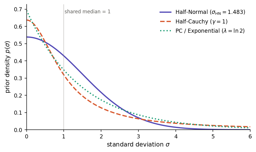
Half-Normal, Half-Cauchy and PC (exponential) priors on a standard deviation σ, each calibrated so that the median equals 1.

Half-Normal(*s*) priors are truncated Gaussians, with density proportional to exp(−σ² / (2 s*²)) for σ ≥ 0. The Gaussian tail decays very fast, so values much larger than *s are effectively ruled out a priori. This makes the prior informative: a misspecified s can bias the posterior SD downward. Use Half-Normal when you have genuine prior information about a plausible upper bound on σ — for example, when σ is on a log-odds scale and values above 5 are implausible on substantive grounds. Chung et al. (2013) recommend Half-Normal specifically to avoid the degenerate σ = 0 estimates produced by penalized-likelihood fits when the number of random-effect groups is small.

Half-Cauchy(γ) priors are truncated Cauchy distributions, with density proportional to 1 / (σ² + γ²). The Cauchy tail decays only polynomially, so even with a small scale γ the prior keeps non-trivial mass at large σ. This is the classical “weakly informative” default recommended by Gelman (2006) for variance components in hierarchical models, and for many years the default in tools such as Stan, rstanarm and brms. The Half-Cauchy is the most permissive of the three: the data can override the prior even when the true SD is large. Its weakness is the flip side of its strength — the tail is so heavy that with few random-effect levels (say, 2–5 groups) the posterior can drift into implausibly large variances and degrade the stability of the INLA grid integration. Use Half-Cauchy when you have many random-effect levels and genuinely want the data to speak for themselves.

PC(*U*, α) priors (Simpson et al., 2017) reduce to an exponential distribution on the standard deviation, p(σ) = λ · exp(−λσ). The functional form is unsurprising; what makes PC priors distinctive is their construction. They are derived from the Kullback–Leibler divergence between the richer model (random effect with SD = σ) and a simpler base model (σ = 0, i.e. no random effect at that level). Deviating from the base model is penalized linearly in its natural Riemannian distance, and this penalty translates into an exponential prior on the SD. The rate λ is set through the interpretable tail-probability statement P(σ > U) = α: you specify a plausible upper bound U and a small probability α of exceeding it, and the software solves λ = −ln(α) / U. PC priors combine the interpretability that Half-Normal lacks (you state a probability rather than an abstract scale parameter) with the robustness that Half-Cauchy can over-supply (exponential tails are lighter than Cauchy, so posterior mass cannot drift arbitrarily far from the null). By construction they shrink the model toward the simpler structure, which is the right behaviour when the random-effect structure is richer than the data can support. For these reasons, PC priors are the default in R-INLA and in Phonometrica.

For routine analyses, keep the PC default. Switch to Half-Cauchy when you have substantive reasons to expect large between-group variability and enough random-effect levels (roughly 10–15 or more) to identify it. Switch to Half-Normal only when you can justify a specific scale on substantive grounds — otherwise its short tail can hide real variance components. When you are unsure, the PC default is the most forgiving choice. It is always good practice to refit with a different prior family as a sensitivity check: posterior summaries that change substantially across priors indicate that the data are too sparse to pin down the variance component, and results should be reported accordingly.

Estimation method

Phonometrica uses INLA-style approximate Bayesian inference (Rue, Martino & Chopin, 2009), not Markov chain Monte Carlo (MCMC). This means that results are available in seconds rather than minutes or hours, with no convergence diagnostics to worry about.

The estimation proceeds differently depending on the model structure:

Fixed-effects models (no random effects, no dispersion parameter): the frequentist MLE is computed first, then a Gaussian posterior approximation is applied by combining the Fisher information with the prior precision. This is exact for Gaussian linear models and highly accurate for GLMs with moderate to large samples.

Mixed-effects models and dispersion families (NB, beta, Student t): the negative log-posterior (likelihood × prior) is optimized directly, with the prior entering the objective function. For mixed-effects models, a two-phase optimization finds the joint posterior mode over fixed effects β and variance parameters θ.

Note

Optimizer dispatch. The outer optimization over variance parameters uses Newton’s method with a finite-difference Hessian (Levenberg–Marquardt damping applied when the Hessian becomes indefinite) for small-dimensional problems, and limited-memory BFGS (Liu & Nocedal 1989) for everything else. The threshold is set at outer dimension 4: random-intercept-only models with one or two grouping factors stay with Newton, while anything with random slopes or multiple crossed random intercepts switches to L-BFGS. Newton’s quadratic convergence is preferred on trivial, well-conditioned surfaces; L-BFGS’s secant-based curvature estimate is preferred on the curved ridges typical of larger models (e.g. a between-cluster fixed effect partially aliased with the corresponding random intercept).

Both optimizers minimize the same Laplace-approximated marginal negative log-likelihood to the same tolerance (10⁻⁸ on the gradient norm), with a secondary function-value convergence criterion for L-BFGS. Log-likelihood values agree across optimizers to within numerical noise (~10⁻¹⁰), far below the threshold at which AIC differences or likelihood-ratio statistics are meaningful. The optimizer used for each fit is reported in the model summary (Converged in N iterations (Newton) or (L-BFGS)) and is accessible from scripts as model.optimizer.

For mixed-effects models, the posterior is then refined via grid integration over the hyperparameters θ (variance component SDs, dispersion parameters). This follows the INLA strategy:

1. A Hessian at the posterior mode defines a Gaussian approximation to the hyperparameter posterior.

2. A central composite design (CCD) grid of evaluation points is constructed in the standardized eigenspace of this Gaussian.

3. At each grid point θ_k, the conditional posterior of the fixed effects β given θ_k is computed, yielding a conditional mean β̂(θ_k) and covariance Σ(θ_k).

4. The results are combined into a mixture-of-Gaussians posterior, with weights proportional to the unnormalized posterior density at each grid point.

This grid integration provides full marginal posteriors for both the fixed effects and the hyperparameters (variance component SDs, dispersion parameters, residual SD), capturing uncertainty from the hyperparameters that a simple plug-in estimate at the mode would miss.

Summary tab (Bayesian mode)

When a Bayesian model is selected, the Summary tab displays posterior summaries instead of frequentist test statistics:

Coefficient table columns:

• Estimate: the posterior mean of each coefficient.

• Est.Error: the posterior standard deviation.

• l-95% CrI / u-95% CrI: bounds of the 95% credible interval. Unlike frequentist confidence intervals, a credible interval has a direct probabilistic interpretation: given the data and the priors, there is a 95% probability that the parameter lies in this range. For mixed-effects models, these are quantiles of the mixture posterior (accounting for hyperparameter uncertainty), not of a single Gaussian.

• pd: the probability of direction, defined as max(P(β > 0), P(β < 0)). This is the Bayesian counterpart to the frequentist p-value. A pd of 0.975 means there is a 97.5% posterior probability that the effect has the same sign as the estimate. Significance codes are based on pd thresholds: *** (pd ≥ 0.999), ** (pd ≥ 0.99), * (pd ≥ 0.975), . (pd ≥ 0.95).

Goodness of fit:

• WAIC (Watanabe–Akaike information criterion): a Bayesian analogue of AIC that estimates the out-of-sample predictive accuracy of the model (Watanabe, 2010; Gelman, Hwang & Vehtari, 2014). Lower WAIC indicates better expected predictive performance. WAIC is reported with its standard error (SE) and the effective number of parameters (p_WAIC), which measures model complexity on the posterior-predictive scale. WAIC is computed from 1000 posterior draws at fit time.

• LPPD (log pointwise predictive density): the sum of the log-predictive densities at each observation, averaged over the posterior. WAIC = −2 × LPPD + 2 × p_WAIC.

• LOO-IC (leave-one-out information criterion): an alternative to WAIC based on Pareto Smoothed Importance Sampling (PSIS-LOO; Vehtari, Gelman & Gabry, 2017). Like WAIC, lower LOO-IC indicates better predictive performance. LOO-IC is reported with its standard error (SE) and the effective number of parameters (p_LOO). LOO-IC is generally preferred over WAIC because it provides per-observation Pareto k diagnostics (see below) that warn when the approximation is unreliable. When all k values are below 0.7, the LOO-IC estimate is considered reliable.

• Pareto k diagnostics: for each observation, a Pareto k value measures the influence of that observation on the posterior. Phonometrica reports a summary of the Pareto k distribution. Values below 0.5 are good, values between 0.5 and 0.7 are acceptable, and values above 0.7 indicate that the LOO-IC estimate for that observation is unreliable — in that case, WAIC may be preferred, or the model should be refit (e.g. with a different family or additional predictors to account for the influential observations).

• Log-marginal likelihood: the Laplace-approximated log p(y | M), which can be used for Bayes factor computation between models.

Hyperparameter posteriors:

For mixed-effects models, the random-effects table reports posterior means and 95% credible intervals for each variance component SD (e.g. sd(Intercept|speaker), sd(residual)), obtained from the grid integration. For families with dispersion parameters, the table also includes the posterior of θ_NB, φ_beta, or σ and ν for Student t.

Note

Posterior mode, mean, and median. For symmetric posteriors (typical with large samples), these three coincide. For small samples or skewed posteriors, they may differ. Phonometrica reports the posterior mean in the coefficient table (as does brms), but all three are stored internally and available via the scripting API. The posterior mode corresponds to the MAP (maximum a posteriori) estimate.

Post-hoc tab (Bayesian mode)

When a Bayesian model is selected, the Post-hoc tab reports estimated marginal means and pairwise contrasts using posterior-based inference:

• CrI (credible intervals) replace confidence intervals in the EMM table.

• pd (probability of direction) replaces adjusted p-values in the contrast table. For each pairwise contrast, pd = Φ(|δ̂/SE|), where δ̂ is the posterior mean of the contrast and SE is its posterior standard deviation.

• No multiplicity adjustment is applied, because pd is not a p-value and the family-wise error rate framework does not apply in the Bayesian context. The Adjustment dropdown is grayed out.

Diagnostics tab (Bayesian mode)

The diagnostic plots work the same way in Bayesian mode, but the residual tests use posterior predictive checking (PPC) instead of frequentist simulation:

1. For each of 200 replicates, a new coefficient vector β^(r) is drawn from the posterior (sampling a grid point with probability proportional to its weight, then drawing from the conditional Gaussian at that grid point).

2. A new response vector is simulated from the model using β^(r) (plus the conditional random-effects modes and dispersion parameters from the sampled grid point).

3. The same KS, dispersion, and outlier test statistics are computed on the simulated data.

4. The proportion of replicates where the simulated test statistic exceeds the observed value is the Bayesian p-value — a measure of how well the model’s predictions match the observed data.

A Bayesian p-value near 0.5 indicates good calibration; values near 0 or 1 indicate systematic discrepancy between the model and the data. Unlike frequentist p-values, these do not reject a null hypothesis; they measure predictive adequacy.

Model comparison (Bayesian mode)

When comparing Bayesian models, the Compare button produces:

• Information criteria table: each model’s WAIC, p_WAIC, LPPD, and SE(WAIC), sorted from best (lowest WAIC) to worst. If LOO-IC is available for all models, the table also includes LOO-IC and p_LOO columns.

• ΔWAIC (and ΔLOO-IC when available): the difference in the information criterion between each model and the best model, with its standard error computed from the pointwise contributions. A model whose ΔIC is within approximately 2 SE of zero is not meaningfully worse than the best model.

• Pareto k summary: when LOO-IC is available, the output includes a summary of the Pareto k diagnostics across all models. If any observation has k > 0.7, a warning is printed advising that the LOO-IC estimate may be unreliable for that model and that WAIC should be preferred.

• Log-marginal likelihood and Bayes factors: for each pair of models, the log Bayes factor is computed as the difference of the log-marginal likelihoods. A log BF > 3 (BF > 20) is conventionally considered strong evidence in favor of the better model.

Frequentist and Bayesian models cannot be compared in the same operation — if you select a mix, Phonometrica will ask you to select only one type.

Note

Interpreting WAIC vs LOO-IC vs AIC. WAIC and LOO-IC are both Bayesian information criteria that estimate out-of-sample predictive accuracy by averaging over the posterior. LOO-IC is generally preferred because it provides per-observation Pareto k diagnostics that flag unreliable estimates. WAIC does not offer such diagnostics, but it is always available (it does not require importance sampling). AIC uses the maximum-likelihood point estimate and does not account for prior regularization or parameter uncertainty. For large samples with weak priors, all three criteria converge. For small samples or informative priors, LOO-IC and WAIC are preferred.

Tips

• Use the Outcome dropdown to match your response variable: Continuous for measurements (e.g. formant frequencies, durations), Continuous (robust) for measurements that may contain outliers or tracking errors, Binary for binary outcomes (e.g. correct/incorrect), Count or Overdispersed count for count data, or Proportion for values between 0 and 1 (e.g. voicing ratios, coarticulation indices, rates of realization). If your proportion data include exact 0s or 1s, consider a small adjustment (e.g. squeezing toward 0.5 by a tiny amount) before fitting, or use Binary as an alternative.

• Start with a simple model and build up complexity. Use Compare to test whether additional terms improve the fit.

• Check the Diagnostics tab after fitting. Poor residual patterns suggest the model may need a different outcome type, additional predictors, or data transformation.

• For vowel formant plots, use the Formant chart checkbox in the EDA tab to reverse both axes.

• When fitting a GAM with speaker or item effects, use s(speaker, bs=re) rather than a fixed effect for the grouping variable. This estimates the between-group variance and shrinks group estimates toward the population mean, reducing overfitting — especially when some groups have few observations. If the effect of a covariate varies by speaker, add a random slope: s(speaker, by=duration, bs=re).

• After fitting a model with a categorical predictor, switch to the Post-hoc tab to see which levels differ from each other. The Holm adjustment (default) controls the family-wise error rate while being more powerful than Bonferroni.

• For interaction models (e.g. F2 ~ frequency * group), use the Trend dropdown in the Post-hoc tab to test whether the slope of a continuous variable differs across groups.

• For mixed-effects models, check Show random effects in the Summary toolbar to inspect the conditional modes (BLUPs) for each speaker, item, or other grouping factor. Large deviations from zero may indicate influential groups worth investigating.

Worked example: formant analysis with a mixed model

Suppose you have a concordance with formant measurements (F1, F2) for several vowels produced by multiple speakers, along with metadata columns for vowel, gender, and speaker.

1. Prepare the data: in the concordance view, use Metric column to compute z-scores on F1 grouped by speaker, then filter out rows where the absolute z-score exceeds 3 to remove outliers. Click Subset to create a clean dataset.

2. Open the analysis: click Analyze in the concordance or dataset toolbar. The analysis view opens with the formula bar at the top and the column list on the left.

3. Build the formula: right-click on F1 and choose Set as response. Double-click on vowel and gender to add them as fixed effects. Right-click on speaker and choose Add as grouping factor to add a random intercept (1|speaker). The formula bar now reads F1 ~ vowel + gender + (1|speaker).

4. Fit the model: make sure the Outcome dropdown is set to Continuous and click Fit. The Summary tab displays the fixed-effects coefficients, the random-effects variance, and goodness-of-fit statistics.

5. Check diagnostics: switch to the Diagnostics tab and select Scaled Residuals vs Fitted. The points should be scattered uniformly between 0 and 1 with no pattern. Check the residual tests below the plot: all three should be non-significant if the model is well-specified.

6. Post-hoc comparisons: switch to the Post-hoc tab, select vowel as the Factor, and click to compute EMMs. The upper table shows the estimated marginal mean of F1 for each vowel; the lower table shows all pairwise contrasts with Holm-adjusted p-values.

7. Compare models: fit a second model without gender (F1 ~ vowel + (1|speaker)), then select both models in the Models panel and click Compare to run a likelihood ratio test.

This same workflow applies to other response types: select Binary for a logistic model of categorical outcomes, Overdispersed count for count data with extra variability (e.g. frequency of schwa deletion per speaker), or Proportion for voicing ratios or similar bounded continuous measures.

References

• Bates, D., Mächler, M., Bolker, B. & Walker, S. (2015). Fitting linear mixed-effects models using lme4. Journal of Statistical Software, 67(1), 1–48.

• Brooks, M.E., Kristensen, K., van Benthem, K.J., Magnusson, A., Berg, C.W., Nielsen, A., Skaug, H.J., Mächler, M. & Bolker, B.M. (2017). glmmTMB balances speed and flexibility among packages for zero-inflated generalized linear mixed modeling. The R Journal, 9(2), 378–400.

• Bürkner, P.-C. (2017). brms: An R package for Bayesian multilevel models using Stan. Journal of Statistical Software, 80(1), 1–28.

• Chung, Y., Rabe-Hesketh, S., Dorie, V., Gelman, A. & Liu, J. (2013). A nondegenerate penalized likelihood estimator for variance parameters in multilevel models. Psychometrika, 78(4), 685–709.

• Dunn, P.K. & Smyth, G.K. (1996). Randomized quantile residuals. Journal of Computational and Graphical Statistics, 5(3), 236–244.

• Ferrari, S.L.P. & Cribari-Neto, F. (2004). Beta regression for modelling rates and proportions. Journal of Applied Statistics, 31(7), 799–815.

• Gelman, A. (2006). Prior distributions for variance parameters in hierarchical models. Bayesian Analysis, 1(3), 515–534.

• Gelman, A., Hwang, J. & Vehtari, A. (2014). Understanding predictive information criteria for Bayesian models. Statistics and Computing, 24(6), 997–1016.

• Hartig, F. (2020). DHARMa: Residual diagnostics for hierarchical (multi-level / mixed) regression models. R package. https://CRAN.R-project.org/package=DHARMa

• Holm, S. (1979). A simple sequentially rejective multiple test procedure. Scandinavian Journal of Statistics, 6(2), 65–70.

• Kristensen, K., Nielsen, A., Berg, C.W., Skaug, H. & Bell, B.M. (2016). TMB: Automatic differentiation and Laplace approximation. Journal of Statistical Software, 70(5), 1–21.

• Lange, K.L., Little, R.J.A. & Taylor, J.M.G. (1989). Robust statistical modeling using the t distribution. Journal of the American Statistical Association, 84(408), 881–896.

• Lenth, R.V. (2016). Least-squares means: the R package lsmeans. Journal of Statistical Software, 69(1), 1–33.

• Nakagawa, S. & Schielzeth, H. (2013). A general and simple method for obtaining R² from generalized linear mixed-effects models. Methods in Ecology and Evolution, 4(2), 133–142.

• Rue, H., Martino, S. & Chopin, N. (2009). Approximate Bayesian inference for latent Gaussian models by using integrated nested Laplace approximations. Journal of the Royal Statistical Society: Series B, 71(2), 319–392.

• Searle, S.R., Speed, F.M. & Milliken, G.A. (1980). Population marginal means in the linear model: an alternative to least squares means. The American Statistician, 34(4), 216–221.

• Simpson, D., Rue, H., Riebler, A., Martino, T.G. & Sørbye, S.H. (2017). Penalising model component complexity: a principled, practical approach to constructing priors. Statistical Science, 32(1), 1–28.

• Tierney, L. & Kadane, J.B. (1986). Accurate approximations for posterior moments and marginal densities. Journal of the American Statistical Association, 81(393), 82–86.

• Vehtari, A., Gelman, A. & Gabry, J. (2017). Practical Bayesian model evaluation using leave-one-out cross-validation and WAIC. Statistics and Computing, 27(5), 1413–1432.

• Watanabe, S. (2010). Asymptotic equivalence of Bayes cross validation and widely applicable information criterion in singular learning theory. Journal of Machine Learning Research, 11, 3571–3594.

• Wood, S.N. (2017). Generalized Additive Models: An Introduction with R (2nd ed.). CRC Press.